Chapter 7 The MVP: Classification Accuracy as a Function of Review Length and Volume
7.1 Introduction
In this notebook I’m trying to build a “minimum viable project” (MVP) that answers the following research questions:
- RQ1: When using a dataset to build a model to predict review ratings based on review sentiment, how does accuracy vary with the number of reviews (volume)?
- RQ2: When using a dataset to build a model to predict review ratings based on review sentiment, how does accuracy vary with the word length of those reviews?
Building on the last section, I will use a logistic regression to create a classification model to predict Yelp reviews’ star ratings based on their sentiment as measured by AFINN. I will divide ratings into positive (“POS”) and negative (“NEG”) reviews, again following Liu (2015)’s recommendation, and use the approaches outlined in Silge and Hvitfeldt (2020) and Silge and Robinson (2020). In some cases I have used examples or hints from websites like Stack Overflow, and I’ve noted that where applicable.
7.2 Preparing the Data
I will again work with the large Yelp dataset available at this link, this time loading the first 500k reviews:
# figure out how to do it reading between the lines of this stackoverflow:
# https://stackoverflow.com/questions/53277351/read-first-1000-lines-from-very-big-json-lines-file-r

yelp_big <- readLines("../tests/data/yelp_academic_dataset_review.json", n = 500000) %>%
  textConnection() %>%
  jsonlite::stream_in(verbose=FALSE)

yelp_big <- yelp_big %>%
  select(stars, text)
Plotting a histogram in Figure 7.1, we see the now-familiar distribution of a slight bump at 1 star followed by an exponential increase towards 5 stars.
yelp_big %>%
  ggplot(aes(x=stars)) +
  geom_histogram(bins=5) +
  labs(
    title = paste0("Large Yelp Dataset (n=",nrow(yelp_big),")"),
    x = "Stars",
    y = "Count") +
  theme_minimal()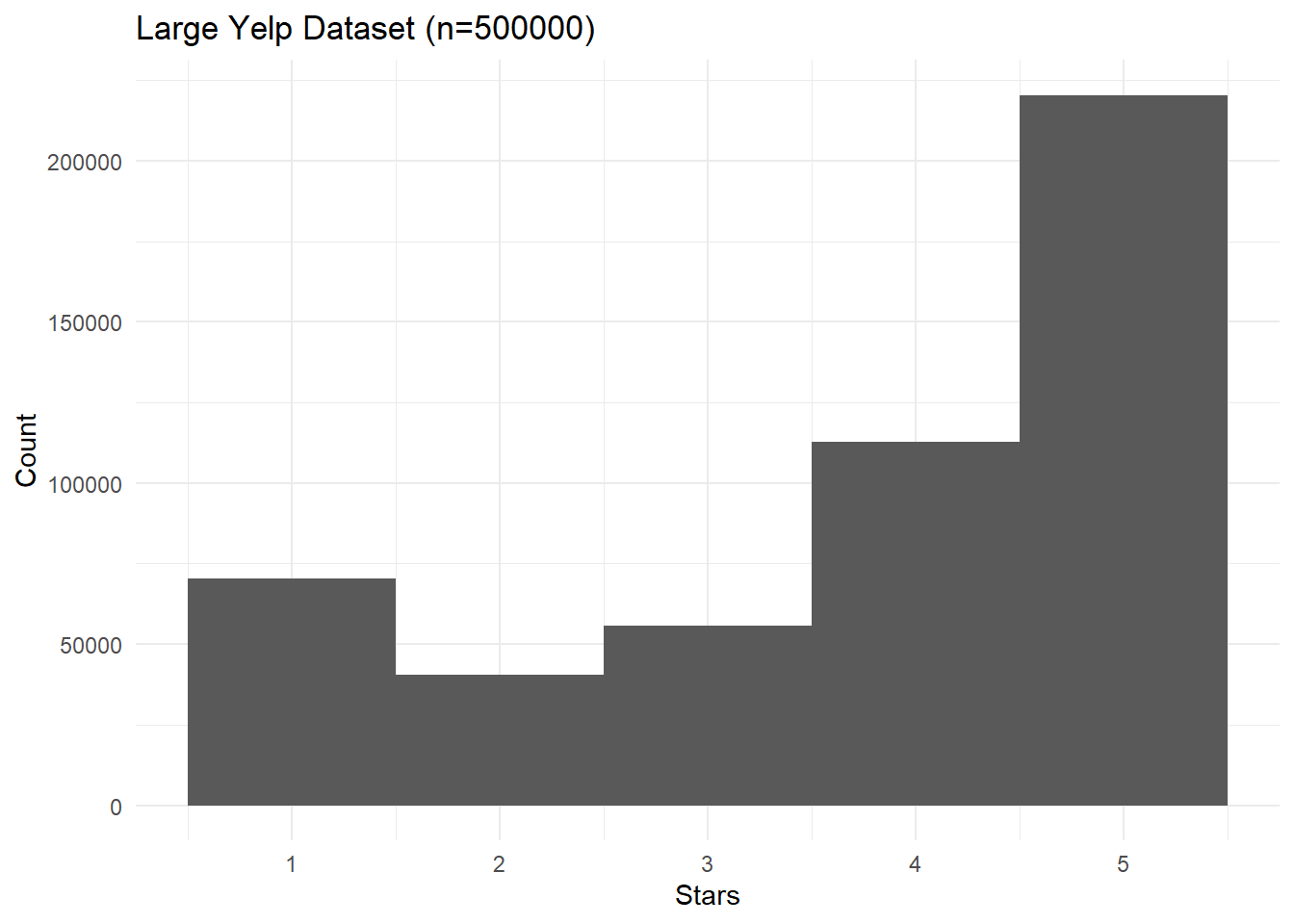
Figure 7.1: Histogram of star ratings for the large Yelp dataset.
Let’s classify the reviews into NEG and POS again, once more classifying reviews with fewer than 3 stars as negative, more than 3 stars as positive, and discarding reviews with 3 stars.
yelp_big_factor <- yelp_big %>%
  mutate(rating_factor = case_when(
    stars < 3 ~ "NEG",
    stars > 3 ~ "POS") %>%
      as.factor()
  ) %>%
  select(-stars) %>%
  drop_na()

yelp_big_factor %>% summary()
## text rating_factor
## Length:444222 NEG:111045
## Class :character POS:333177
## Mode :characterSince we found that classification didn’t work well with an unbalanced dataset, we will downsample the dataset so that we have the same number of positive and negative reviews.
set.seed(1234)
yelp_balanced <- yelp_big_factor %>%
  filter(rating_factor == "NEG") %>%
  bind_rows(yelp_big_factor%>%
              filter(rating_factor == "POS") %>%
              slice_sample(n=yelp_big_factor %>% filter(rating_factor == "NEG") %>% nrow() ))

yelp_balanced %>% summary()
## text rating_factor
## Length:222090 NEG:111045
## Class :character POS:111045
## Mode :characterLet’s try AFINN again on the balanced set. First we’ll get the AFINN sentiments for all our reviews.
tic()
afinn_yelp_big <- yelp_balanced %>%
  rowid_to_column() %>%
  tidytext::unnest_tokens(word, text) %>%
  left_join(afinn) %>%
  group_by(rowid) %>%
  summarise(afinn_sent = sum(value, na.rm = T))
toc()
## 71.83 sec elapsedyelp_big_bal_afinn <- afinn_yelp_big %>%
left_join(yelp_balanced %>% rowid_to_column()) %>%
select(-rowid)The density plot in Figure 7.2 shows that NEG and POS reviews still have overlapping but different distributions in this dataset, which suggests that our model might reasonably be able to tell them apart.
yelp_big_bal_afinn %>%
  ggplot(aes(x=afinn_sent, fill=rating_factor)) +
  geom_density(alpha=0.5) +
  labs(#title = "Density Distributions of AFINN Sentiment for POS and NEG Reviews",
    title = paste0("Large Balanced Yelp Dataset (n=",nrow(yelp_big_bal_afinn),")"),
    x = "AFINN Sentiment",
    y ="Density",
    fill="Sentiment") +
  theme_minimal()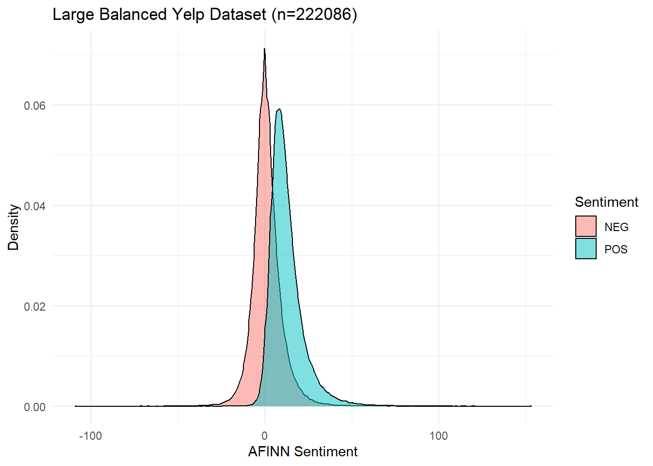
Figure 7.2: Density Distributions of AFINN Sentiment for POS and NEG Reviews.
We will now compute the word length for each review so we can see how review length affects our predictions. As we can see in Figure 7.3, most of our reviews are quite short–roughly 200,0000 are under 250 words–but a few extend beyond 1000 words.
wordcounts_yp <- yelp_big_bal_afinn %>%
  select(text) %>%
  rowid_to_column() %>%
  tidytext::unnest_tokens(word, text) %>%
  group_by(rowid) %>%
  summarise(n = n()) %>%
  arrange(n)  %>%
  mutate(id = 1,
         cumdist = cumsum(id))

wordcounts_yp %>%
  ggplot() +
  geom_point(aes(y=cumdist, x=n)) +
  theme_minimal() +
  labs(title =paste0("Large Yelp Dataset (n=",nrow(yelp_big_bal_afinn),")"), #: Cumulative Distribution of Word-Lengths",
       x = "Word Length",
       y = "# of Reviews")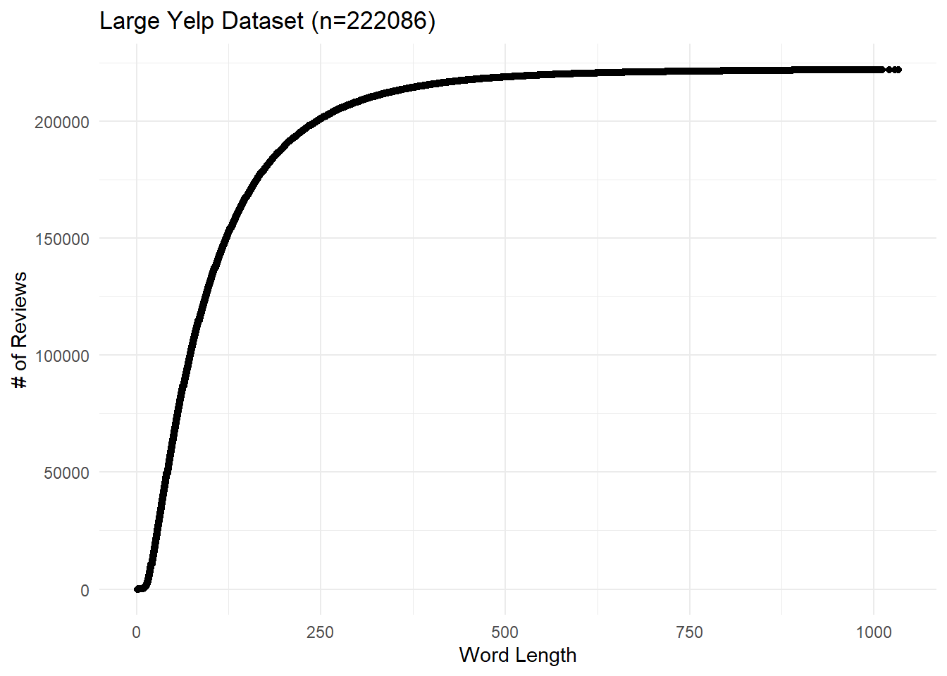
Figure 7.3: Large Yelp Dataset: Cumulative distribution of word lengths.
Next we’ll join the word-length column to our balanced Yelp dataset, completing the pre-processing.
7.3 Experiment 1: Logistic Regression on Globally Balanced Data
In this section we will look at how review length and volume affect classification accuracy using a logistic regression based on review sentiment. I will divide the data into \(n\) non-overlapping subsets based on their lengths, and then I will divide those subsets into \(n\) overlapping subsets of increased size, and then will run a logistic regression on each of these latter subsets. The output will be an \(n\times n\) matrix plotted as a heat map where each cell represents model accuracy for a given number of reviews with lengths within a given range.
More precisely, here are the steps I will follow:
- Choose a number of quantiles \(n\), and divide reviews into \(n\) quantiles by word length.
- Find how many reviews are in each quantile. Take the smallest total number of reviews \(mintotal\): for comparability, this is the largest number of reviews we will consider.
- Within each quantile, consider \(n\) overlapping subsets of increasing size ranging from \(mintotal/n\) to \(mintotal\).
- For each quantile, for each group of reviews, run a logistic regression to predict review ratings and log its accuracy.
After some initial experimentation, I’ve chosen to use \(n=5\) quantiles since it gives us a good number of subsets of reasonable size.
First, we set up a function to run a logistic regression on an arbitrary dataset and return the prediction accuracy. This is a functionized version of the code I used earlier.
do_logit <- function (dataset) {

  # for a train/test split: get a random vector as long as our dataset that is 75% TRUE and 25% FALSEe.
  index <- sample(c(T,F),
                  size = nrow(dataset),
                  replace = T,
                  prob=c(0.75,0.25))

  # extract train and test datasets by indexing our dataset using our random index
  train <- dataset[index,]
  test <- dataset[!index,]

  # use `glm()` to run a logistic regression predicting the rating factor based on the AFINN score.
  logit <- glm(data= train,
               formula= rating_factor ~ afinn_sent,
               family="binomial")

  pred <- predict(logit,
                  newdata = test,
                  type="response")

  # now predict the outcome based on whichever has the greater probability, find out if each prediction is correct, and compute the accuracy
  test_results <- test %>%
    bind_cols(tibble(pred = pred)) %>%
    mutate(pred = if_else(pred > 0.5, "POS", "NEG")) %>%
    mutate(correct = if_else (pred == rating_factor, T, F)) %>%
    summarise(accuracy = sum(correct) / nrow(.)) %>%
    unlist()

  return (test_results)
}
It’s not quite “tidy,” but we can run this analysis easily with two nested for loops. Here I break the reviews into 5 quantiles by word length, and then break each quantile down into 5 overlapping subsets of increasing length.
# for reproducibility, set the random number generator seed
set.seed(1234)

# how many quantiles?
num_qtiles <- 5

# get the limits of the word-quantiles for display purposes
qtiles <- quantile(yelp_data$words, probs = seq(0, 1, (1/num_qtiles)))

# find the word-quantile for each review using the fabricatr::split_quantile() function
yelp_data <- yelp_data %>%
  mutate(qtile = fabricatr::split_quantile(words,
                                           type=num_qtiles))

# get the number of reviews in the smallest quantile.
# we're going to use this to compare groups of the same/similar size.
minn <- yelp_data %>%
  group_by(qtile) %>%
  summarise(n = n()) %>%
  summarise(minn = min(n)) %>%
  unlist()

# set up an empty results tibble.
results <- tibble()

# boolean flag: will we print updates to the console?
# I used this for testing but it should be disabled in the final knit
verbose <- FALSE

tic()
# Consider each quantile of review word lengths one at a time
for (word_qtile in 1:num_qtiles){
  # within each quantile of reviews broken down by length, consider several different numbers of reviews
  for (num_qtile in 1:num_qtiles){

    # number of reviews we will consider in this iteration.
    num_reviews <- num_qtile * minn/num_qtiles

    # message for me to keep track
    if (verbose == TRUE) {
      message (paste0("Considering ", num_reviews, " reviews with word length in the range (",qtiles[[word_qtile]],",",qtiles[[word_qtile+1]],")"))
    }

    # filter the rows we want: the right number of words, and the right number of reviews, then run a logistic regression on them
    data_for_logit <- yelp_data %>%
      filter(qtile==word_qtile) %>%
      slice_sample(n = num_reviews)

    # get true percentage of positives, so we can look at sample balance
    pct_true_pos <- data_for_logit %>%
      summarise(n = sum(rating_factor == "POS") / nrow(.)) %>%
      unlist()

    # run the logistic regression on our data
    result <- data_for_logit %>%
      do_logit()

    # add our result to our results tibble. this wouldn't be best practice for thousands of rows, but it's fine here.
    results <- bind_rows(
      results,
      tibble(word_qtile = word_qtile,
             num_qtile = num_qtile,
             accuracy = result,
             pct_true_pos = pct_true_pos)
    )
  }
}
toc()
## 2.75 sec elapsedThe code runs quickly (<5s on my machine) and gives some interesting-looking results shown below in Figure 7.4. First, all of the accuracy metrics are quite high: our success rates ranged from around 80% to 86%. But interestingly, it looks like we get better results from shorter reviews!
results %>%
  ggplot() +
  geom_tile(aes(x=word_qtile, y=num_qtile, fill=accuracy)) +
  scale_x_continuous(breaks = 1:num_qtiles,
                     labels = paste0("Q",1:num_qtiles,": ",qtiles, "-",lead(qtiles)) %>% head(-1)) +
  scale_y_continuous(breaks = 1:num_qtiles,
                     labels = (1:num_qtiles * minn/num_qtiles)) +
  labs(x = "Review Word Length by Quantile",
       y = "Number of Reviews",
       fill = "Accuracy")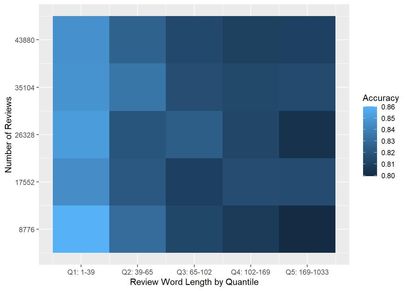
Figure 7.4: Heat map of logistic regression prediction accuracy for the large balanced Yelp dataset.
However, before drawing conclusions we should look more closely at the data. As we can see below in Figure 7.5, there is a big difference in each quantile’s true positive rate. And based just on visual inspection, it looks like higher true positive rates in Figure 7.5 are correlated with higher prediction accuracy rates in Figure 7.4.
results %>%
  ggplot() +
  geom_tile(aes(x=word_qtile, y=num_qtile, fill=pct_true_pos)) +
  scale_x_continuous(breaks = 1:num_qtiles,
                     labels = paste0("Q",1:num_qtiles,": ",qtiles, "-",lead(qtiles)) %>% head(-1)) +
  scale_y_continuous(breaks = 1:num_qtiles,
                     labels = (1:num_qtiles * minn/num_qtiles)) +
  labs(x = "Review Word Length by Quantile",
       y = "Number of Reviews",
       fill = "True Positive Rate")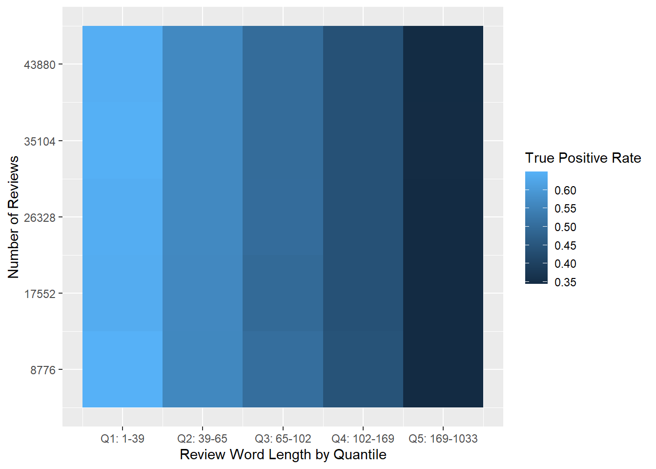
Figure 7.5: Heat map of the percentage of true positive reviews in each quantile.
We can confirm this intuition by plotting each subset’s true positive rate versus its quantile, as shown in Figure 7.6. We can see very strong correlation between the two variables. This correlation casts some doubt on the apparent results in Figure 7.4, since we know from a previous experiment that an imbalanced dataset can lead to wonky predictions. Are we really seeing that shorter reviews lead to more accurate predictions, or are we actually seeing that datasets with higher true positive rates are easier to classify? There’s no easy way to disentangle this.
results %>%
  ggplot(aes(x = word_qtile, y  =pct_true_pos)) +
  geom_point() +
  labs(x =  "Review Word Length by Quantile",
       y = "True Positive Rate") +
    scale_x_continuous(breaks = 1:num_qtiles,
                     labels = paste0("Q",1:num_qtiles,": ",qtiles, "-",lead(qtiles)) %>% head(-1)) +
  theme_minimal()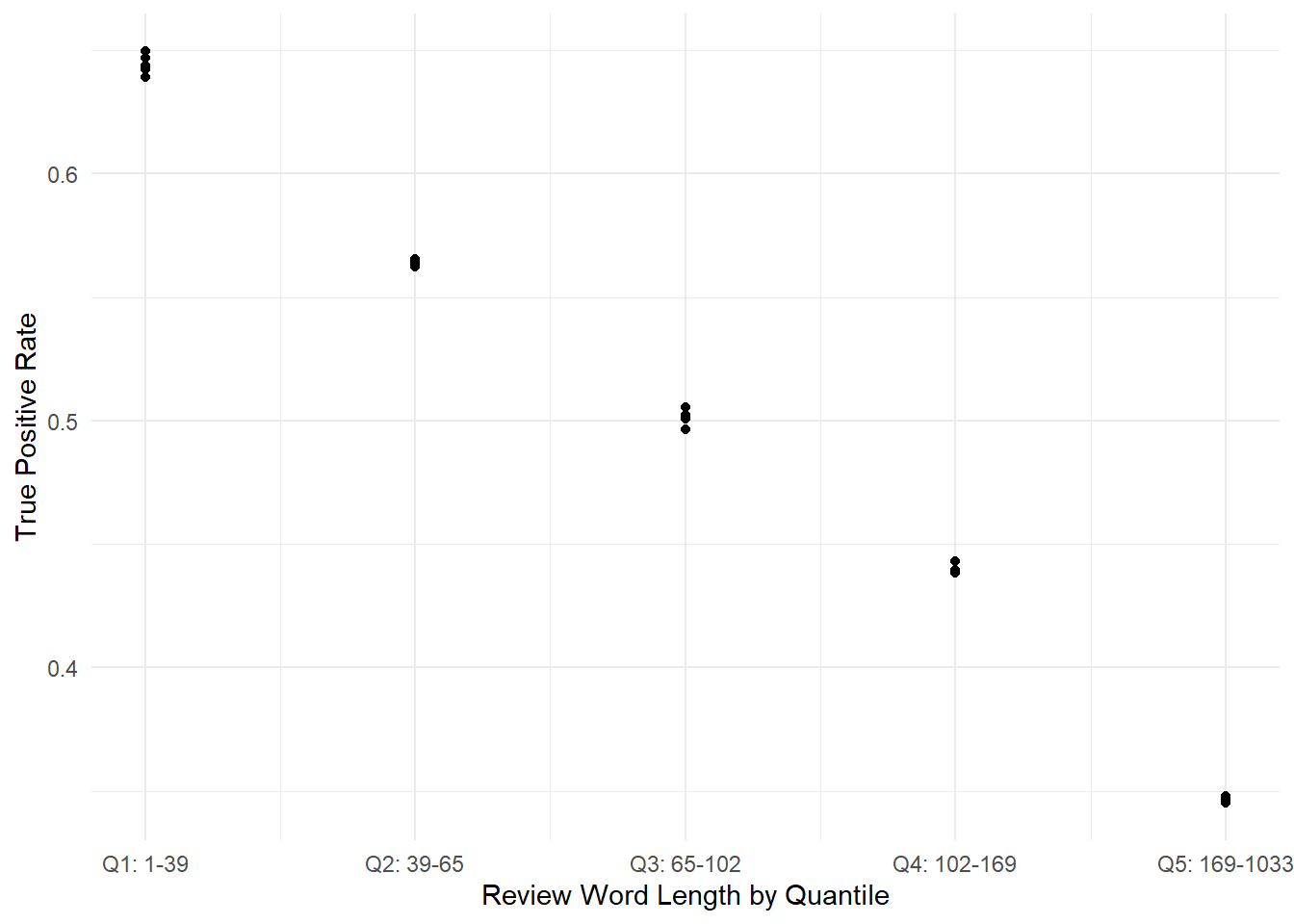
Figure 7.6: True positive rates vs. review lengths for each subset, showing strong correlation.
However, since our predictions were reasonably accurate (80%-86%) across a wide range of true-positive rates (0.35-0.65), we can draw one positive preliminary conclusion from this experiment:
Preliminary Conclusion: Logistic regression based on AFINN sentiment provides an accurate (>80%) method of predicting review sentiment on datasets across a wide range of word lengths, review counts, and true-positive rates.
This is good news, but the confounding effect of the true-positive rates means we don’t have a direct answer to our original question of how accuracy varies with review length and volume. This will require some additional processing so that we can operate on a collection of balanced sub-sets.
7.4 Experiment 2: Logistic Regression on Micro-Balanced Data
In this experiment, I will address the correlation between each data subset’s true-positive rate and review length by further balancing each subset. This probably has a technical name, but here I will call it “micro-balancing.” The rest of the algorithm will be the same.
Recall that in Experiment 1 above, we found that our data sub-sets were imbalanced between positive and negative reviews. This suggests that reviews tend to differ in length according to their sentiment, and as we can see in Figure 7.7, negative reviews do tend to be longer than positive reviews.
yelp_data %>%
  filter(rating_factor == "POS") %>% pull(words) %>% ecdf() %>%
  plot(col="green",
       main = "ECDF for POS (green) and NEG (red) reviews",
       xlab = "Review Length",
       ylab = "Proportion")
yelp_data %>%
  filter(rating_factor == "NEG") %>% pull(words) %>% ecdf() %>% lines(col="red")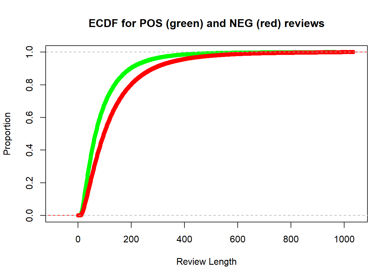
Figure 7.7: Empirical cumulative distribution function for lengths of positive and negative reviews.
The simplest approach is to further downsample the data so that each subset is of the same size and balanced between positive and negative reviews. The following code block runs largely the same analysis as in Experiment 1, except this time I balance each data subset by downsampling before running through a logistic regression. To ensure that all samples are the same size, I first find the smallest number of positive or negative reviews in any subset. Then, in each step of the analysis I randomly downsample the positive and negative reviews to have exactly this many entries.
# for reproducibility, set the random number generator seed
set.seed(1234)

# how many quantiles?
num_qtiles <- 5

# get the limits of the word-quantiles for display purposes
qtiles <- quantile(yelp_data$words, probs = seq(0, 1, (1/num_qtiles)))

# find the word-quantile for each review using the fabricatr::split_quantile() function
yelp_data <- yelp_data %>%
  mutate(qtile = fabricatr::split_quantile(words,
                                           type=num_qtiles))

# get the number of reviews in the smallest subset of BOTH rating and length quintile.
# we're going to use this to compare groups of the same/similar size.
minn <- yelp_data %>%
  group_by(qtile, rating_factor) %>%
  summarise(n = n()) %>%
  ungroup() %>%
  summarise(minn = min(n)) %>%
  unlist()
## `summarise()` regrouping output by 'qtile' (override with `.groups` argument)# set up an empty results tibble.
results <- tibble()
# boolean flag: will we print updates to the console?
# I used this for testing but it should be disabled in the final knit
verbose <- FALSE
tic()
# Consider each quantile of review word lengths one at a time
for (word_qtile in 1:num_qtiles){
# within each quantile of reviews broken down by length, consider several different numbers of reviews
for (num_qtile in 1:num_qtiles){
# number of reviews we will consider in this iteration.
num_reviews <- num_qtile * minn/num_qtiles
# message for me to keep track
if (verbose == TRUE) {
message (paste0("Considering ", num_reviews*2, " reviews with word length in the range (",qtiles[[word_qtile]],",",qtiles[[word_qtile+1]],")"))
}
# I'm doing this in two steps to keep it simple, since we need to get the same number of positive and negative reviews.
# First, filter the positive rows we want: the right number of words, and the right number of reviews
data_pos <- yelp_data %>%
filter(qtile == word_qtile) %>%
filter(rating_factor == "POS") %>%
slice_sample(n = num_reviews)
# Then filter the negative rows we want:
data_neg <- yelp_data %>%
filter(qtile == word_qtile) %>%
filter(rating_factor == "NEG") %>%
slice_sample(n = num_reviews)
# then combine the positive and negative rows.
data_for_logit <- bind_rows(data_pos, data_neg)
# get true percentage of positives, so we can look at sample balance
pct_true_pos <- data_for_logit %>%
summarise(n = sum(rating_factor == "POS") / nrow(.)) %>%
unlist()
# run the logistic regression on our data
result <- data_for_logit %>%
do_logit()
# add our result to our results tibble. this wouldn't be best practice for thousands of rows, but it's fine here.
results <- bind_rows(
results,
tibble(word_qtile = word_qtile,
num_qtile = num_qtile,
accuracy = result,
pct_true_pos = pct_true_pos)
)
}
}
toc()## 2.63 sec elapsedAlthough the additional downsampling takes a bit more time, the code still runs quickly (<10s on my machine). However, before looking at the results let’s confirm that each data subset was balanced between positive and negative reviews. Figure 7.8 below shows that the data subsets were balanced, so we can look at our prediction accuracy without worrying about unbalanced data affecting our results.
results %>%
  ggplot() +
  geom_tile(aes(x=word_qtile, y=num_qtile, fill=pct_true_pos)) +
  scale_x_continuous(breaks = 1:num_qtiles,
                     labels = paste0("Q",1:num_qtiles,": ",qtiles, "-",lead(qtiles)) %>% head(-1)) +
  scale_y_continuous(breaks = 1:num_qtiles,
                     labels = (2*round(1:num_qtiles * minn/num_qtiles))) +
  labs(x = "Review Word Length by Quantile",
       y = "Number of Reviews",
       fill = "True Positive Rate")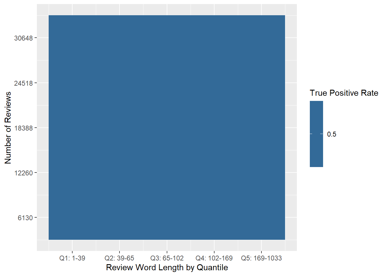
Figure 7.8: Heat map of the percentage of true positive reviews in each quantile of the micro-balanced dataset.
The results shown below in Figure 7.9 are promising. The accuracy metrics are still quite high, and range from around 79% to around 83%. This is a bit worse overall than in Experiment 1, but we can be more confident now that these are real results and not an artefact of any underlying imbalance in the data.
results %>%
  ggplot() +
  geom_tile(aes(x=word_qtile, y=num_qtile, fill=accuracy)) +
  scale_x_continuous(breaks = 1:num_qtiles,
                     labels = paste0("Q",1:num_qtiles,": ",qtiles, "-",lead(qtiles)) %>% head(-1)) +
  scale_y_continuous(breaks = 1:num_qtiles,
                     labels = (2*round(1:num_qtiles * minn/num_qtiles))) +
  labs(x = "Review Word Length by Quantile",
       y = "Number of Reviews",
       fill = "Accuracy")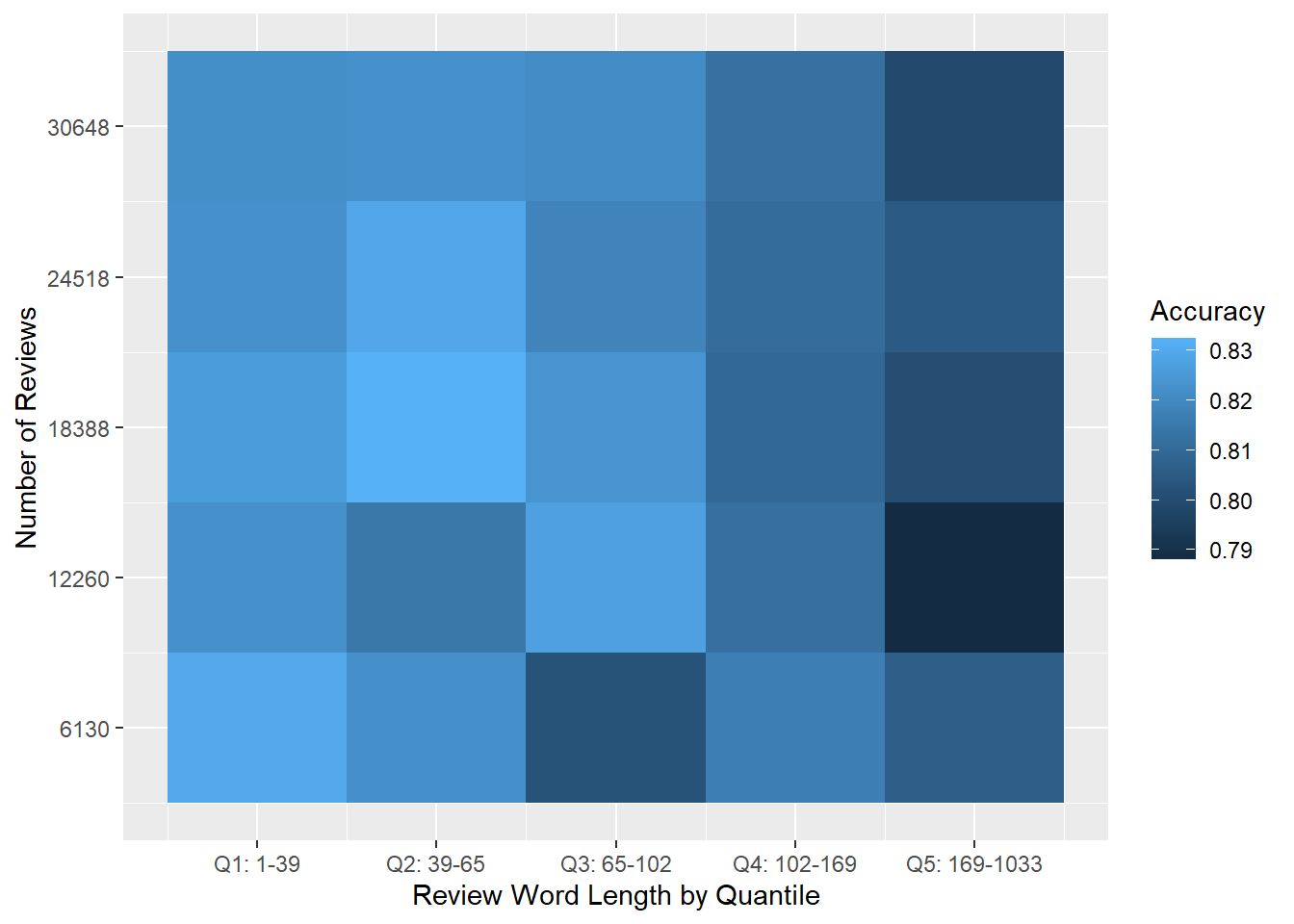
Figure 7.9: Heat map of logistic regression prediction accuracy for the micro-balanced Yelp dataset.
We’re now in a position to draw some conclusions from our analysis.
First, shorter reviews are effective for predicting ratings, and the longest reviews are the least effective. We can see this trend clearly in Figure 7.10 below, where the first three quintiles perform reasonably well, but then accuracy degrades quickly in Q4 and Q5. We can hypothesize about why this might be. For example, shorter reviews might have more “information density” and longer reviews might tend to ramble on and be “noisier.” It’s much easier to get the gist of “This place sucks, I hate it” than it is of an 800-word essay that begins “Upon entering the establishment, I was first greeted by an aroma of…”
results %>%
  ggplot() +
  geom_boxplot(aes(x=as.factor(word_qtile), y = accuracy)) +
  theme_minimal() +
  scale_x_discrete(breaks = 1:num_qtiles,
                     labels = paste0("Q",1:num_qtiles,": ",qtiles, "-",lead(qtiles)) %>% head(-1)) +
  labs(x = "Review Word Length by Quantile",
       y = "Accuracy")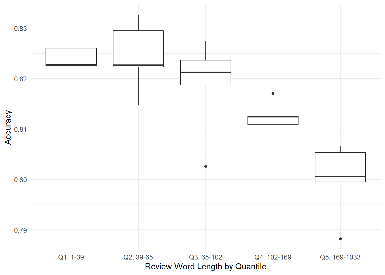
Figure 7.10: Experiment 2: Boxplots of review accuracy by word-length quintile.
Second, our results were not dependent on the number of reviews, and we achieved good accuracy with even a modest number of reviews. Figure 7.11 shows the distribution of model accuracy according to the number of reviews, and the distributions overlap substantially. There is no clear trend here, suggesting that this approach to classification doesn’t benefit from having more than on the order of 10,000 input reviews.
results %>%
  ggplot() +
  geom_boxplot(aes(x=as.factor(num_qtile), y = accuracy)) +
  theme_minimal() +
  scale_x_discrete(breaks = 1:num_qtiles,
                     labels = (2*round(1:num_qtiles * minn/num_qtiles))) +
  labs(x = "Number of Reviews",
       y = "Accuracy")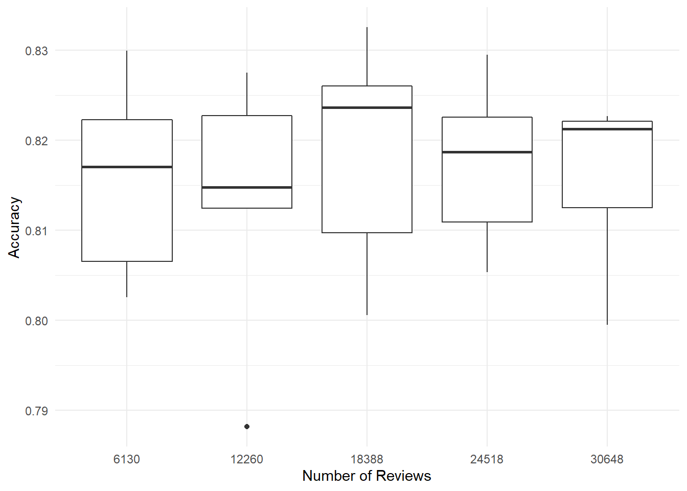
Figure 7.11: Experiment 2: Boxplots of review accuracy by number of reviews.
If one were so inclined, one could also demonstrate this with a stylish Joy-Division-style ridge-density plot.
results %>%
  ggplot() +
  ggridges::geom_density_ridges(aes(x = accuracy, y=as.factor(num_qtile)))  +
  theme_minimal() +
  scale_y_discrete(breaks = 1:num_qtiles,
                     labels = (2*round(1:num_qtiles * minn/num_qtiles))) +
  labs(y = "Number of Reviews",
       x = "Accuracy")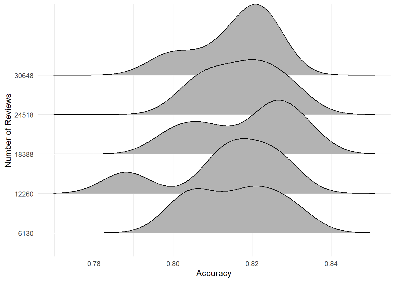
Figure 7.12: Experiment 2: Shameless pandering to the ref with a ‘Joy Division’ ridge plot of review accuracy by number of reviews.
If one were a stickler for parametric statistics, one might want to see this lack of correlation demonstrated with a linear regression. Here I will run a linear regression to predict a model’s accuracy from the number of reviews it considers.
##
## Call:
## lm(formula = accuracy ~ num_qtile, data = results)
##
## Residuals:
##       Min        1Q    Median        3Q       Max
## -0.027484 -0.006335  0.002200  0.007103  0.016486
##
## Coefficients:
##              Estimate Std. Error t value Pr(>|t|)
## (Intercept) 0.8148239  0.0053016 153.695   <2e-16 ***
## num_qtile   0.0004102  0.0015985   0.257      0.8
## ---
## Signif. codes:  0 '***' 0.001 '**' 0.01 '*' 0.05 '.' 0.1 ' ' 1
##
## Residual standard error: 0.0113 on 23 degrees of freedom
## Multiple R-squared:  0.002855,   Adjusted R-squared:  -0.0405
## F-statistic: 0.06586 on 1 and 23 DF,  p-value: 0.7997
As expected, the volume of reviews is not a statistically significant predictor of accuracy: the p-value for the num_qtile variable is 0.8, the p-value for the model overall is roughly 0.8, and the Adjusted \(R^2\) is negative(!). My results show no statistical evidence that, over these ranges, the number of input reviews is associated with a model’s accuracy.
7.5 Conclusions
In this section I ran two experiments to predict a Yelp review’s rating based on its AFINN sentiment using logistic regression. In each experiment, I built and evaluated 25 models using subsets of my data with different word lengths and numbers of reviews. I demonstrated that you can get good accuracy (~80%) with a relatively small number of reviews (~10,000) using a simple sentiment-detection algorithm (AFINN) and a simple classification model (logistic regression).
In Experiment 1 I balanced my overall dataset between positive and negative reviews by random down-sampling. However, I found that my subsets were unbalanced, and found furthermore that the degree of imbalance was strongly correlated with accuracy. Still, I noted that the overall accuracy was still quite good across the entire range of imbalance, and so one interpretation is that this method is quite robust on unbalanced datasets.
In Experiment 2 I balanced each subset to have approximately the same number of positive and negative reviews, again using random down-sampling. Using these “micro-balanced” datasets, I derived the following answers to my two research questions:
- A1: Review accuracy was better with shorter reviews, and the longest reviews were the least effective.
- A2: Review accuracy was not correlated with the number of reviews used as inputs, provided the number of reviews is on the order of 10,000.
Results in Experiment 2 were very good overall: accuracy ranged from around 79% to around 83% across all models.
7.6 Next Steps
- Consider evaluating model performance across the entire dataset, not just the testing component of the subset used to generate the model. For discussion.K
- Consider a more complex sentiment-detection algorithm.
- Consider a more complex classification engine, e.g. Naive Bayes Classifier using text tokens instead of a real-valued sentiment score.
7.7 SessionInfo
## R version 4.0.2 (2020-06-22)
## Platform: x86_64-w64-mingw32/x64 (64-bit)
## Running under: Windows 10 x64 (build 18363)
##
## Matrix products: default
##
## locale:
## [1] LC_COLLATE=English_Canada.1252  LC_CTYPE=English_Canada.1252    LC_MONETARY=English_Canada.1252 LC_NUMERIC=C                    LC_TIME=English_Canada.1252
##
## attached base packages:
## [1] stats     graphics  grDevices utils     datasets  methods   base
##
## other attached packages:
##  [1] vip_0.2.2         glmnet_4.0-2      Matrix_1.2-18     ggridges_0.5.2    discrim_0.1.1     tictoc_1.0        textrecipes_0.3.0 lubridate_1.7.9   yardstick_0.0.7   workflows_0.2.0
## [11] tune_0.1.1        rsample_0.0.8     recipes_0.1.13    parsnip_0.1.4     modeldata_0.0.2   infer_0.5.3       dials_0.0.9       scales_1.1.1      broom_0.7.0       tidymodels_0.1.1
## [21] tidytext_0.2.5    forcats_0.5.0     stringr_1.4.0     dplyr_1.0.2       purrr_0.3.4       readr_1.3.1       tidyr_1.1.1       tibble_3.0.3      ggplot2_3.3.2     tidyverse_1.3.0
##
## loaded via a namespace (and not attached):
##  [1] colorspace_1.4-1   ellipsis_0.3.1     class_7.3-17       fs_1.5.0           rstudioapi_0.11    listenv_0.8.0      furrr_0.1.0        farver_2.0.3       SnowballC_0.7.0
## [10] prodlim_2019.11.13 fansi_0.4.1        xml2_1.3.2         codetools_0.2-16   splines_4.0.2      knitr_1.29         jsonlite_1.7.0     pROC_1.16.2        packrat_0.5.0
## [19] dbplyr_1.4.4       compiler_4.0.2     httr_1.4.2         backports_1.1.7    assertthat_0.2.1   cli_2.0.2          htmltools_0.5.0    tools_4.0.2        gtable_0.3.0
## [28] glue_1.4.1         naivebayes_0.9.7   rappdirs_0.3.1     Rcpp_1.0.5         cellranger_1.1.0   DiceDesign_1.8-1   vctrs_0.3.2        iterators_1.0.12   timeDate_3043.102
## [37] gower_0.2.2        xfun_0.16          stopwords_2.0      globals_0.13.0     rvest_0.3.6        lifecycle_0.2.0    future_1.19.1      MASS_7.3-51.6      ipred_0.9-9
## [46] hms_0.5.3          parallel_4.0.2     yaml_2.2.1         gridExtra_2.3      rpart_4.1-15       stringi_1.4.6      highr_0.8          tokenizers_0.2.1   foreach_1.5.0
## [55] textdata_0.4.1     lhs_1.0.2          hardhat_0.1.4      shape_1.4.5        lava_1.6.8         rlang_0.4.7        pkgconfig_2.0.3    evaluate_0.14      lattice_0.20-41
## [64] labeling_0.3       tidyselect_1.1.0   fabricatr_0.10.0   plyr_1.8.6         magrittr_1.5       bookdown_0.20      R6_2.4.1           generics_0.0.2     DBI_1.1.0
## [73] pillar_1.4.6       haven_2.3.1        withr_2.2.0        survival_3.1-12    nnet_7.3-14        janeaustenr_0.1.5  modelr_0.1.8       crayon_1.3.4       utf8_1.1.4
## [82] rmarkdown_2.3      usethis_1.6.1      grid_4.0.2         readxl_1.3.1       blob_1.2.1         reprex_0.3.0       digest_0.6.25      webshot_0.5.2      munsell_0.5.0
## [91] GPfit_1.0-8        viridisLite_0.3.0  kableExtra_1.1.0
7.8 References
References
Liu, Bing. 2015. Sentiment Analysis: Mining Opinions, Sentiments, and Emotions. Cambridge: Cambridge University Press. https://doi.org/10.1017/CBO9781139084789.
Silge, Julia, and Emil Hvitfeldt. 2020. Supervised Machine Learning for Text Analysis in R. https://smltar.com/.
Silge, Julia, and David Robinson. 2020. Text Mining with R: A Tidy Approach. O’Reilly. https://www.tidytextmining.com/index.html.