Chapter 8 Beyond the MVP: Looking at Longer Reviews

8.1 Introduction

In this notebook I’ll dig deeper into the last section’s strange finding that longer reviews generated worse predictions. Recall that we used a logistic regression to create a classification model to predict Yelp reviews’ star ratings based on their sentiment as measured by AFINN. After evaluating 25 models using data subsets with review lengths and volumes, the two main results were:

• A1: Review accuracy was better with shorter reviews, and the longest reviews were the least effective.
• A2: Review accuracy was not correlated with the number of reviews used as inputs, provided the number of reviews is on the order of 10,000.

Here I’ll test two hypotheses:

• H1: The presence of negators like “but” and “not” are associated with both incorrect predictions and with increasing review length.
• H2: Decreasing readability scores are associated with both incorrect predictions and with increasing review length.

The intuition is twofold: first, that AFINN’s simple “bag-of-words” approach can’t capture complex sentence structures; and second, that the number of complex sentence structures will tend to increase as the length of a review increases. As a result, we would expect more complex reviews to have worse predictions using a simple model based on AFINN scores.

8.2 Results from the Previous Section

I will again work with the large Yelp dataset available at this link. For brevity I’m omitting the code here (see the previous section or .Rmd source file), but the code:

• Loads the first 500k reviews;
• Converts integer star ratings to NEG and POS factors;
• Balances the NEG and POS reviews using random downsampling;
• Calculates each review’s AFINN sentiment score; and
• Calculates each review’s word length.

In the last section we found that prediction accuracy was better with shorter texts and poor with longer texts. To give a fairer analysis of the model and to smooth out any potential for us to get poor results by chance, here I extend the analysis a bit to run the model 30 times for each data subset–randomly resampling a test/train split each time–and computing the average accuracy across all trials. The results are similar to what we found in the last section and are shown below in Figure 8.1. Accuracy ranges from around 79% to around 83%, and it looks like results are worse for longer reviews.

results_oldmodel %>%
  ggplot() +
  geom_tile(aes(x=word_qtile, y=num_qtile, fill=accuracy)) +
  scale_x_continuous(breaks = 1:num_qtiles, 
                     labels = paste0("Q",1:num_qtiles,": ",qtiles, "-",lead(qtiles)) %>% head(-1)) +
  scale_y_continuous(breaks = 1:num_qtiles,
                     labels = (2*round(1:num_qtiles * minn/num_qtiles))) +
  labs(x = "Review Word Length by Quantile",
       y = "Number of Reviews",
       fill = "Accuracy")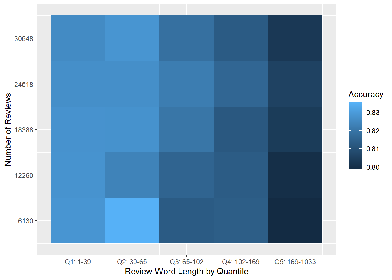

Figure 8.1: Overview of results: Heat map of logistic regression prediction accuracy for the micro-balanced Yelp dataset. Each cell shows average accuracy for 30 tests on random samples.

This trend is clear in Figure 8.2 below, where the first three quintiles perform reasonably well, but then accuracy degrades quickly in Q4 and Q5.

results_oldmodel %>%
  ggplot() +
  geom_boxplot(aes(x=as.factor(word_qtile), y = accuracy)) +
  theme_minimal() +
  scale_x_discrete(breaks = 1:num_qtiles, 
                     labels = paste0("Q",1:num_qtiles,": ",qtiles, "-",lead(qtiles)) %>% head(-1)) +
  labs(x = "Review Word Length by Quantile",
       y = "Accuracy")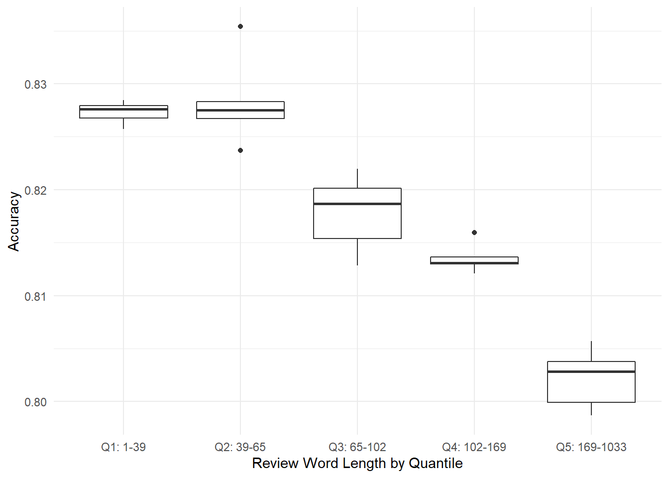

Figure 8.2: Experiment 2: Boxplots of review accuracy by word-length quintile, showing the worst performance with the longest reviews. Each point is an average of model results based on 30 random samples within the subset.

8.3 Finding Misclassified Reviews

We’ll modify our logistic regression function so that it returns its prediction for each review, not only the accuracy for the whole set of reviews.

logit_predict <- function (dataset) {

  # for a train/test split: get a random vector as long as our dataset that is 75% TRUE and 25% FALSEe.
  index <- sample(c(T,F), 
                  size = nrow(dataset),
                  replace = T,
                  prob=c(0.75,0.25))
  
  # extract train and test datasets by indexing our dataset using our random index
  train <- dataset[index,]
  test <- dataset[!index,]
  
  # use `glm()` to run a logistic regression predicting the rating factor based on the AFINN score.
  logit <- glm(data= train,
               formula= rating_factor ~ afinn_sent,
               family="binomial")
  
  pred <- predict(logit, 
                  newdata = test,
                  type="response")
  
  # now predict the outcome based on whichever has the greater probability, find out if each prediction is correct
  test_results <- test %>%
    bind_cols(tibble(pred = pred)) %>%
    mutate(pred = if_else(pred > 0.5, "POS", "NEG")) %>%
    mutate(correct = if_else (pred == rating_factor, T, F)) 
  
  return (test_results)
}

For this analysis, we will look at the largest set of the longest reviews that we considered in the previous section. This code takes the full set of the longest reviews, downsamples it so that there are the same number of positive and negative reviews, and then fits a logistic regression to a training subset and returns predictions for a test subset.

set.seed(1234)
word_qtil <- 5
minnnum_reviews <- 5 * minn/num_qtiles 
   # I'm doing this in two steps to keep it simple, since we need to get the same number of positive and negative reviews.
    # First, filter the positive rows we want: the right number of words, and the right number of reviews
    data_pos <- yelp_data %>%
      filter(qtile == word_qtile) %>%
      filter(rating_factor == "POS") %>%
      slice_sample(n = num_reviews)
    
    # Then filter the negative rows we want:
    data_neg <- yelp_data %>%
      filter(qtile == word_qtile) %>%
      filter(rating_factor == "NEG") %>%
      slice_sample(n = num_reviews)
    
    # then combine the positive and negative rows.
    data_for_logit <- bind_rows(data_pos, data_neg) 
    
    # run the logistic regression on our data
    predictions <- data_for_logit %>%
      logit_predict()

We’ll use this new dataset for the rest of this section.

8.4 Qualitative Analysis of Misclassified Reviews

Let’s begin by looking at a few misclassified reviews in detail. Table 8.1 shows a review that was actually positive, but was predicted to be negative. Although it says a lot of positive-valence words like “epic” and “nice,” it also uses negative-valence words like “desperate,” “chintzy,” and “cheesy” that balance out for an overall AFINN score of just 8. A human reader can tell that the reviewer introduces these negative words just to dismiss them (as in “Feels modern and not too cheesy”), but AFINN just sees these words and scores them as negative.

predictions[7,]$text %>% 
  knitr::kable(col.names = "Review Text (True Pos, Misclassified)",
               caption="True positive misclassified as negative. Note the number of negative-valence words like 'cheesy.'") %>%
  kableExtra::kable_styling(bootstrap_options = "striped")

Table 8.1: True positive misclassified as negative. Note the number of negative-valence words like ‘cheesy.’

Review Text (True Pos, Misclassified)

First and foremost, I want to say that the people watching here is EPIC. Beyond that, it’s pretty nice for a casino. Feels modern and not too cheesy although it’s kind of hard to have a casino and NOT have some chintzy decor. Also, this casino doesn’t quite have that “desperate” feeling that a lot of other, older, established casinos seem to have. I’m not a gambler so I won’t speak to the gaming aspect of things but I think this casino does a good job of drawing people in who aren’t looking to lose money at the slots and would prefer to drop their hard-earned cash at a bar. The bar areas here are loungy and well laid out and it doesn’t feel like everyone who works at the casino is giving you the stinkeye bc you want to sit down somewhere that isn’t connected to a machine or at a table. I could totally see myself coming in here to grab a drink or two before venturing on to some other bar.

Table 8.2 shows a true negative review that was misclassified as positive. The reviewer uses many positive-valence words like “quality,” and uses few negative-valence words. Again the positive-valence words are negated or muted by modifiers (“medium-quality lamb”), but AFINN can’t detect this subtlety.

set.seed(1233)
predictions %>%
  filter(pred=="POS" & correct==FALSE) %>%
  slice_sample(n=1) %>% 
  select(text) %>%
 knitr::kable(col.names = "Review Text (True Neg, Misclassified)",
              caption="True negative misclassified as positive. Note the number of positive-valence words like 'quality' and 'good,' and the relative absence of negative-valenec words like 'bad' or 'unpleasant.'" ) %>%
  kableExtra::kable_styling(bootstrap_options = "striped")

Table 8.2: True negative misclassified as positive. Note the number of positive-valence words like ‘quality’ and ‘good,’ and the relative absence of negative-valenec words like ‘bad’ or ‘unpleasant.’

Review Text (True Neg, Misclassified)

I feel trolled by fellow Yelpers and IG foodies for thinking that James Cheese would be a great dinner choice. This is one of those cases where it looks good, but doesn’t taste good and I’m not afraid to call it as it is, despite the impeccable service that we got. Taste should come before presentation and service, sorry. I would describe a meal at James Cheese as a waste of a cheat day. Go do AYCE sushi instead. We got the kimchi fries, coconut pineapple drink and the signature ribs platter in mild and medium. The kimchi fries were a bit dry and not nearly as good as the ones from Banh Mi Boyz, although kudos for the meat. It was just dry while at the same time soggy with kimchi juice. There wasn’t a discernable difference between the mild and medium ribs and both are overly sweet. The combo of ribs, mozzarella cheese, corn, scrambled eggs, hotdogs, and kimchi seems so mismatched. I would go so far to call out that anyone who gave this restaurant more than 3 stars not a real foodie. Please, I want to eat real good food, bonus if it looks good.

As a final check, let’s look at the true-negative review with the highest AFINN score to see where AFINN went most wrong. Table 8.3 shows this review, which received an AFINN score of 113 despite being negative. The author here also uses positive-valence words with negating words (e.g. “I wasn’t particularly impressed”), which confuses AFINN and leads to a high score. In addition, the author does just have a lot of nice things to say about the meal, which even I find a bit confusing.

predictions %>%
  filter(correct==FALSE) %>%
  arrange(desc(afinn_sent)) %>%
  head(1) %>%
  select(text) %>%
  mutate(text = gsub("\n", " ", text)) %>%
  knitr::kable(col.names = "Review Text",
               caption = "This review was a true negative, but because it is very long it has a very high AFINN score of 113.") %>%
  kableExtra::kable_styling(bootstrap_options = "striped")

Table 8.3: This review was a true negative, but because it is very long it has a very high AFINN score of 113.

Review Text

Tastefully decorated with wine bottles, glasses, and interesting lighting fixtures, the interior feels open and bright thanks to floor-to-ceiling windows. A fantastic outdoor back patio includes an outdoor bar and lounge areas. The service was pleasant and patient - We were given a bread basket with crispy flat bread seasoned with tarragon and a few slices of white bread. It was accompanied with a rather plain marinara sauce, which foreshadowed the upcoming meal. Baby Red Romaine & Escarole Salad Cara Cara orange, fennel, shaved Parmigiano-Reggiano and old wine vinaigrette A light start of fresh lettuce, a slightly tart vinaigrette, ripe Cara Cara orange, and cheese. While the orange and the dressing was enjoyable, something was left to be desired…perhaps it’s because of my unrefined wine and cheese palette, but I wasn’t particularly impressed. Memorable Summerlicious starter salads include the butterleaf truffle salad at Truffles at the Four Seasons (which has since closed) and Tutti Matti’s carpaccio salads. Bigeye Tuna Tartare & Spicy Sopressata Cracked olives, garlic grissini, arugula, lemon and Sicilian organic extra virgin olive oil Fresh tuna tartare on a bed of salami was a welcome dish, especially since I’ve never tried sopressata before. The saltyness of the cured ham paired with the freshnesses of the tuna created an interesting balance between bites. The olives were typical, and the bread sticks brought a crunch but no flavour to the plate. Perhaps if they were toasted a bit more or rolled in sesame, it would’ve been a nice compliment to the dish. Wild & Tame Mushroom Soup Six kinds of mushrooms (no butter or cream) Thick, warm, and hearty - this had the rich texture of a comforting soup despite the lack of cream or butter. I was impressed with the consistency and I love the taste of mushrooms so I thoroughly enjoyed this soup. As with the salad, there was something lacking - the “wow” factor that I always hope for at ’licious restaurants. The best mushroom soup that I’ve tasted was Wild Mushroom Soup from Tutti Matti - unfortunately not on their current menu. Grilled Top Sirloin Fettina Charred onion, heirloom tomato and rocket salad with crumbled Gorgonzola The vegetables were nice and warm, and the sauce surrounding the steak sweet however the steak wasn’t particularly interesting or great. Tender and nicely cooked, it was a good, simple cut of sirloin but didn’t blow me away or leave a lasting impression on my palette. Grilled Jail Island Salmon Pickled summer beets, heirloom carrots, watercress salad and horseradish crème fraîche Despite my half-success with the fish at Biff’s Bistro, I decided that it was worth another go. While tasty, I’m quickly getting bored with this Summerlicious lunch. The beets were nice, warm, and soft and the horseradish crème fraîche had great flavour. However the salmon was…just salmon. Roasted Portobello Mushroom & Brie Quesadilla Caramelized onions, pico de gallo, chipotle crema, plantain tortilla chips and cilantro cress My personal favourite of the entrées, the chipotle cream had a tangy flavour that tasted great with the pico de gallo and quesadilla. The pico de gallo (salsa) was ripe and simple. Always a fan of portobello, these quesadillas had great flavour. While an interesting visual, the tortilla chips were lacking the flavour I usually enjoy from plantains. As a plantain chip lover, they were a disappointment. I’d rather crack open a bag of the Samai Plantain chips that I got addicted to Barbados. Chocolate Toffee Crunch Cheesecake Dulce de leche cream Thick cheesecake that was more toffee-like than chocolate. The caramel was pleasant with the dense cake. I wasn’t a fan of the bit of toffee that accompanied the cake but overall I’d say that this was the best dessert out of the three. Bavarian Vanilla Cream Ontario strawberry compote and dark cherry balsamic Nice and warm with a smooth texture, the vanilla cream dessert sat on one of the better compotes that I’ve tried. I found myself scooping this dessert up more for the compote than the cream. Coconut Rum Baba Tropical fruit salad and banana cream This spongy cake was covered with coconut shavings over pineapple, mango, and lychee. A sweet, generous drizzle of rum syrup soaked into the cake quite nicely. While I wasn’t the biggest fan of this dessert initially, over time as I enjoyed my company it grew on me. It wasn’t too rich or filling. Wonderfully designed and decorated, Jump Café & Bar creates a vibrant, young, and upscale environment quite well. I would return for a drink at the bar, and the service was fantastic. However, I thought it was missing that the “oomph” factor that would make me wholeheartedly recommend this restaurant for future Summerlicious romps. This is a good spot to take someone who wants a very simple no-frills meal.

In addition, this shows a potential source of error when using raw AFINN scores: there is no weighting for review length. A review that makes 50 lukewarm statements will be rated 50 times more positive than a shorter review that only makes one. As Figure 8.3 shows, there does seem to be a positive correlation between a review’s word length and its AFINN score. It may therefore be worth looking at normalizing AFINN scores, either to word length or number of sentences, to see if we can improve our accuracy.

yelp_data %>%
  ggplot(aes(x=words, y=afinn_sent)) +
  geom_point() +
  geom_smooth(method="lm", formula = y~x) +
  theme_minimal() +
  labs(x="Words",
       y="AFINN Sentiment")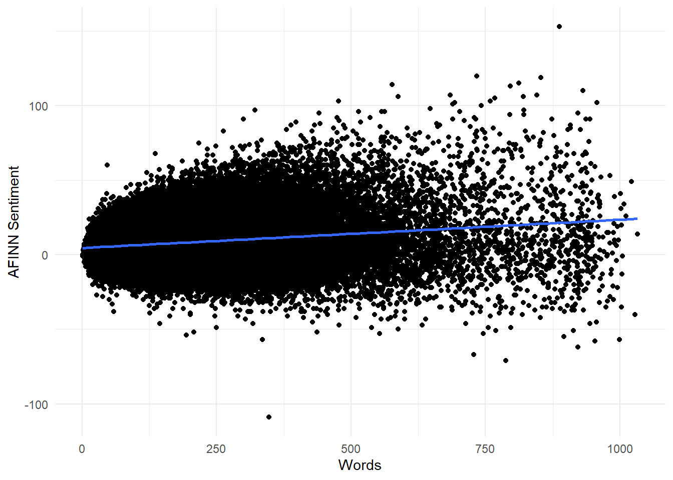

Figure 8.3: Longer reviews seem to have slightly higher AFINN sentiment scores on average, and it also looks like variance increases with word length.

lm_fit <- lm(data = yelp_data, formula = afinn_sent ~ words)

lm_fit %>% broom::tidy() %>%
  knitr::kable(
    caption = "Results from a linear regrssion predicting AFINN sentiment from review length in words. Although the $R^2$ is low, the model shows good statistical significance."
  )

Table 8.4: Results from a linear regrssion predicting AFINN sentiment from review length in words. Although the \(R^2\) is low, the model shows good statistical significance.

term	estimate	std.error	statistic	p.value
(Intercept)	4.5909815	0.0322987	142.14137	0
words	0.0190131	0.0002022	94.02087	0

We can draw two conclusions from this (mostly) qualitative look at misclassified reviews:

• Misclassified reviews often use many opposite-valence words but negate them using words like “but” or “not.”
• The most-misclassified review by AFINN score was extremely long, suggesting that normalizing AFINN scores by review length might improve our accuracy.

8.5 Negations

Let’s investigate the effects of negations/negators in our review texts. It’s possible, for example, that misclassified reviews could tend to have more negators like “not” or “but.” Since AFINN is a pure bag-of-words approach it can’t distinguish between “I am happy this is very good” and “I am not happy this is not very good.” Accounting for negators might therefore give us a way to capture this information and improve our predictions.

8.5.1 Negations and Prediction Accuracy

Let’s look at “but”s and “nots” in the correct vs incorrect predictions.

predictions <- predictions %>%
  mutate(buts = stringr::str_count(text, "but "),
         nots = stringr::str_count(text, "not "),
         buts_nots = buts + nots)

The average numbers or buts and nots are different:

predictions %>%
  group_by(correct) %>%
  summarise(avg_negs = mean(buts_nots)) %>%
  knitr::kable()

correct	avg_negs
FALSE	3.703857
TRUE	3.370872

Let’s look more closely at the number of negators in correctly and incorrectly predicted reviews. Table 8.5 below shows the results of three two-sided t-tests comparing the average number of “buts”, “nots”, and combined “buts & nots” for correct and incorrect predictions. While “buts” and “buts & nots” differ significantly, the difference in the number of “nots” is not statistically significant at the standard level of \(p<0.05\). The other two results show strong significance.

pred_bn <- predictions %>%
  t_test(buts_nots ~ correct) %>%
  mutate(measure = "buts & nots")

pred_b <- predictions %>%
  t_test(buts ~ correct) %>%
  mutate(measure = "buts")

pred_n <- predictions %>%
  t_test(nots ~ correct) %>%
  mutate(measure = "nots")

bind_rows(pred_bn,
          pred_b,
          pred_n) %>%
  select(measure, statistic, t_df, p_value, alternative) %>%
  knitr::kable(caption = "Results for two-sided t-tests for equivalence of means in the numbers of 'nots', 'buts', and 'nots and buts' in correct and incorrect predictions for the subset of longer reviews.")

Table 8.5: Results for two-sided t-tests for equivalence of means in the numbers of ‘nots’, ‘buts’, and ‘nots and buts’ in correct and incorrect predictions for the subset of longer reviews.

measure	statistic	t_df	p_value	alternative
buts & nots	3.934286	2026.129	0.0000863	two.sided
buts	4.564349	2092.784	0.0000053	two.sided
nots	1.875926	2024.922	0.0608092	two.sided

This suggests that negators might play a role in lowering our model’s accuracy, and that accounting for negators somehow might improve our predictions.

8.5.2 Negations and Word Length

Let’s look at the number of negations vs. word length for the longer reviews. Figure 8.4 below shows that the number of “buts” and “nots” tends to increase with word length.

predictions %>%
  ggplot(aes(x=words, y=buts_nots)) +
  geom_point(position = "jitter") +
  geom_smooth(method = "lm", se = FALSE) +
  theme_minimal()+
  labs(x = "# Words",
       y = "# buts and nots")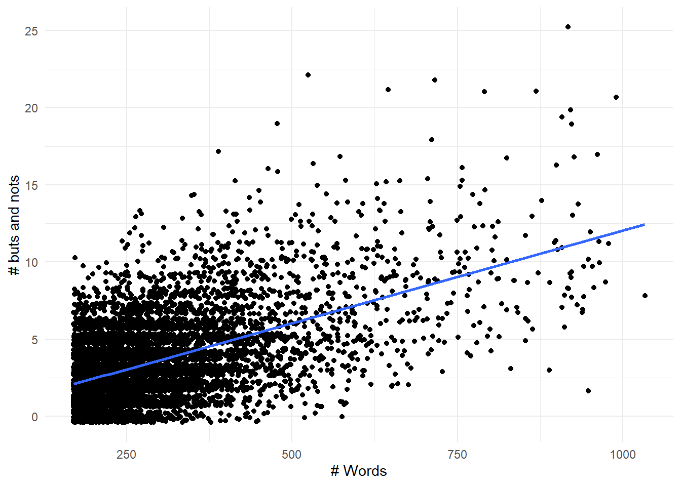

Figure 8.4: The combined number of ‘buts’ and ‘nots’ tends to increase as reviews get longer.

A linear regression shows that this association is strongly significant, with both model and coefficient p-values below \(2^{-16}\). The \(R^2\) is 0.295, which looks reasonable based on the plot.

lm(data = predictions, formula = buts_nots ~ words) %>%
  summary()

## 
## Call:
## lm(formula = buts_nots ~ words, data = predictions)
## 
## Residuals:
##    Min     1Q Median     3Q    Max 
## -9.403 -1.546 -0.288  1.263 15.672 
## 
## Coefficients:
##              Estimate Std. Error t value Pr(>|t|)    
## (Intercept) 0.0563061  0.0648218   0.869    0.385    
## words       0.0119693  0.0002105  56.867   <2e-16 ***
## ---
## Signif. codes:  0 '***' 0.001 '**' 0.01 '*' 0.05 '.' 0.1 ' ' 1
## 
## Residual standard error: 2.283 on 7719 degrees of freedom
## Multiple R-squared:  0.2953, Adjusted R-squared:  0.2952 
## F-statistic:  3234 on 1 and 7719 DF,  p-value: < 2.2e-16

We can conclude that “buts” and “nots” are associated with both incorrect predictions and with increasing word lengths.

8.6 Readability

In this section we’ll look at how a review’s readability relates to model accuracy. We’ll use the sylcount package’s readability() function to calculate Flesch-Kincaid (FK) readability scores and see how they interact with accuracy. FK scores are a common way to measure a text’s complexity and will be familiar to anyone who uses Microsoft Word. Without going into details, texts with higher FK scores are assumed to be easier to read.

predictions_re <- predictions %>%
  pull(text) %>%
  sylcount::readability() %>%
  select(-words) %>%
  bind_cols(predictions, .)

Figure 8.5 shows FK readability ease vs. word length:

predictions_re %>%
  ggplot(aes(x=words, y=re)) +
  geom_point() +
  theme_minimal() +
  labs(x = "# Words",
       y = "Flesch-Kincaid Reasing Ease Score")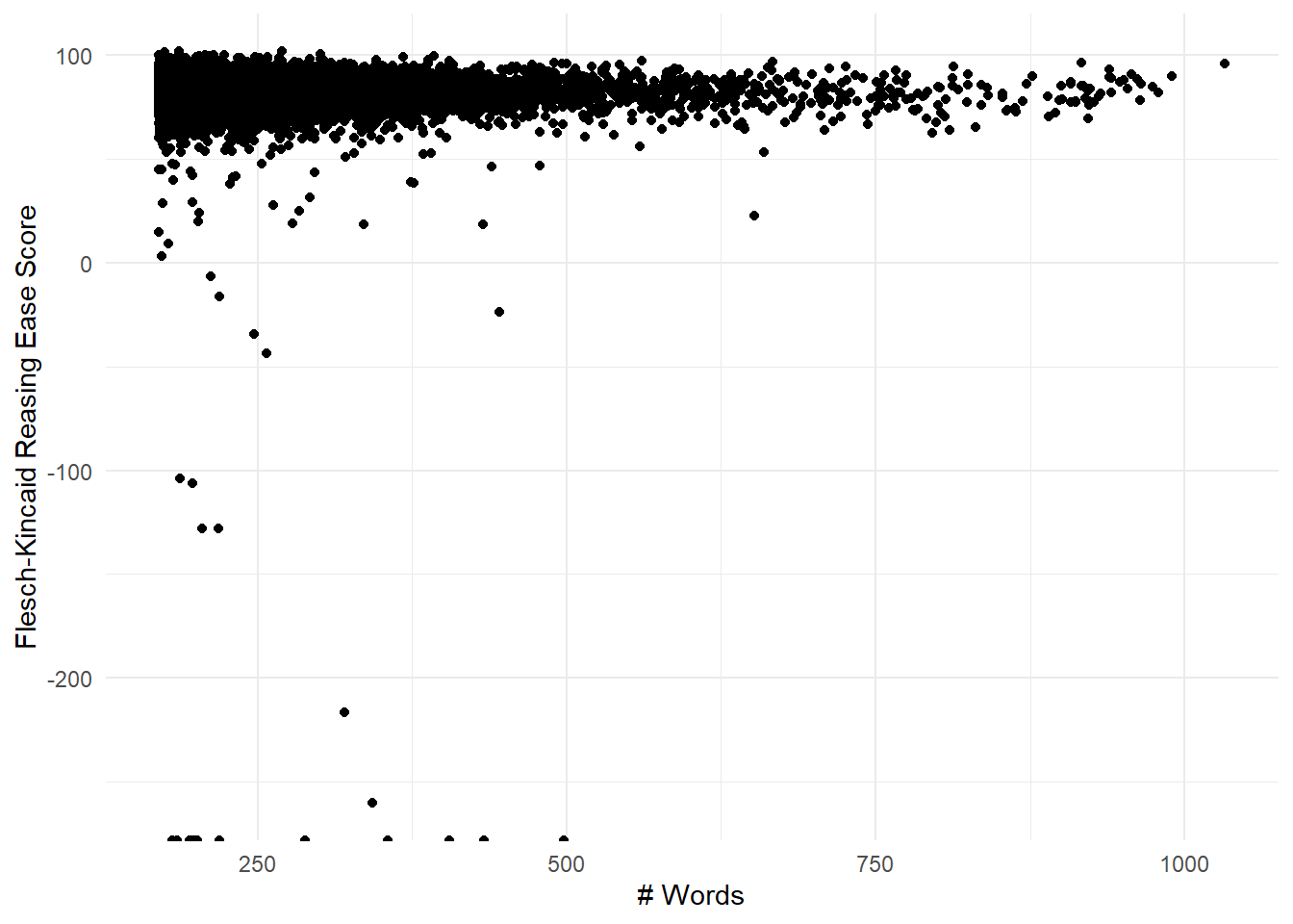

Figure 8.5: FK reading ease for the original set of long reviews. While most scores are between 0 and 100, there are many outliers as low as -250.

We immediately see that the FE index has no theoretical minimum value, and this is a problem. Let’s look at the shortest super low one to see what’s going on. Looks like these reviewers use " . " instead of “.” so the algorithm thinks it’s all one sentence.

predictions_re %>%
  filter( re == min(re)) %>%
  filter(words == min(words)) %>%
  pull(text) %>%
  stringr::str_trunc(150)

## [1] "Leaving it 2 stars the food was bland the Greek fries were a little dry nothing special about the gyro but not uneatable . Also a bit over priced 1..."

So we’ll fix this by replacing " ." with “.” and try again. Results are shown below in Figure 8.6.

predictions_re <- predictions %>%
  mutate(text = stringr::str_replace_all(text,  " \\.", "\\."))  %>%
  pull(text) %>%
  sylcount::readability() %>%
  select(-words) %>%
  bind_cols(predictions, .)

predictions_re %>%
  ggplot(aes(x=words, y=re)) +
  geom_point() +
  theme_minimal() +
  labs(x = "# Words",
       y = "Flesch-Kincaid Reasing Ease Score")

Figure 8.6: FK reading ease for the set of long reviews with non-standard period breaks removed. Note there are still many low outliers.

Since there are still many low outliers, the new shortest least-readable review is presented below in Table 8.6. We can see two things: first, it’s honestly full of run-on sentences; and second, it looks like the reviewer is using carriage returns as sentence markers. We can fix the second item by replacing carriage returns with periods.

predictions_re %>%
  filter(re == min(re)) %>%
         filter(words == min(words)) %>%
  pull(text) %>%
  stringr::str_trunc(500) %>%
  knitr::kable(col.names = "Shortest Least-Readable Review",
               caption = "Statistics for two-sided t-tests comparing the number of correct and incorrect predictions based on the number of nots, buts, and nots & buts they contain.")

Table 8.6: Statistics for two-sided t-tests comparing the number of correct and incorrect predictions based on the number of nots, buts, and nots & buts they contain.

Shortest Least-Readable Review
My review not to criticise people personally but the business when we booked they said that they will pick us 6:15 am from our hotel so we waited almost half an hours extra outside the hotel till the picked us up

Then we spend more time till they distribute us to another busses and kept asking if we would like to upgrade the seat or the bus for extra money we waste one and a half hours until we hit the road the busses was not so good very old no USB to charge phone because we where thinking… |

As can be seen in Figure 8.7, there are still very low readability scores after fixing these “errors” in the dataset. This suggests that many reviews have inherent features, like run-on sentences, that result in genuinely low FK scores.

predictions_re <- predictions %>%
  mutate(text = stringr::str_replace_all(text,  " \\.", "\\."),
         text = stringr::str_replace_all(text, "\\s*\\n\\s*", ". "))  %>%
  pull(text) %>%
  sylcount::readability() %>%
  select(-words) %>%
  bind_cols(predictions, .)

predictions_re %>%
  ggplot(aes(x=words, y=re)) +
  geom_point() + 
  theme_minimal() +
  labs(x = "# Words",
       y = "Flesch-Kincaid Reasing Ease Score")

Figure 8.7: FK reading ease for the set of long reviews with non-standard period breaks and carriage returns removed. Outliers persist.

Note that we have one value that has -Inf readability! This review, included as Table ?? below, has a lot of text but no sentence-ending punctuation so it breaks the readability algorithms. We will filter this entry out in the rest of this section.

predictions_re %>%
  filter(re == -Inf) %>%
  pull(text) %>%
  stringr::str_trunc(300) %>%
  knitr::kable(col.names = "Infinitely Unreadable Review")

Infinitely Unreadable Review
Well not a good experience so got approved for credit threw Conns and was happy for that they delivered the furniture day just like they,said so I get back home and see they didn’t set the tv up ok so I call my brother over we set the tv up on the stand and the tv doesn’t work what a surprise …

So let’s again now look at readability and prediction accuracy. The boxplots for the distributions look quite similar, as can be seen below in Figure 8.8.

predictions_re %>%
  filter(re > -Inf) %>%
  ggplot() +
  geom_boxplot(aes(x=as.factor(correct), y=re)) +
  theme_minimal() +
  labs(x = "Prediction Accuracy",
       y = "Flesch-Kincaid Reasing Ease Score")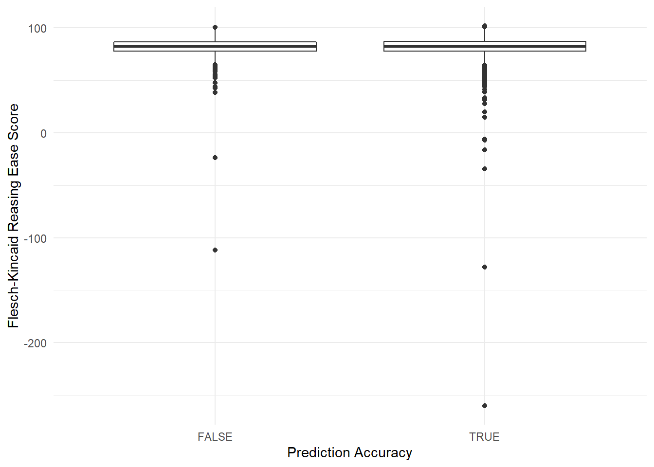

Figure 8.8: Distributions of FK reading ease scores for reviews with correct and incorrect predictions. The boxplots are very similar.

Looking at the sample means, they’re not so different (after removing the one value of -Inf!)

predictions_re %>%
  group_by(correct) %>%
  filter(re > -Inf) %>%
  summarise(avg_re = mean(re)) %>%
  knitr::kable()

correct	avg_re
FALSE	81.77320
TRUE	81.85309

And a two-sided t-test does not show statistical evidence that the distribution means are different.

predictions_re %>%
  filter(re > -Inf) %>%
  t_test(re ~ correct) %>%
  knitr::kable()

statistic	t_df	p_value	alternative	lower_ci	upper_ci
-0.2975279	2157.305	0.7660922	two.sided	-0.6064841	0.4466979

To sum up, I found two problems with using readability measures on this data. First, many texts use either non-standard sentence breaks (e.g. " . " or carriage returns) which confuses the algorithms. But even after fixing these data issues, many texts have little or no punctuation at all. Readability algorithms rely on sentence counts, so they won’t work on informal texts without conventional punctuation.

So readability is not associated with prediction accuracy in this sample of longer reviews.

8.7 Summing Up So Far

Let’s do a quick recap on what we’ve learned so far in this section:

• Misclassified reviews often use many opposite-valence words but negate them using words like “but” or “not.”
• The most-misclassified review by AFINN score was extremely long, suggesting that normalizing AFINN scores by review length might improve our accuracy.
• Negators like “buts” and “nots” are associated with both incorrect predictions and with increasing word lengths.
• Readability is not associated with prediction accuracy in this sample of longer reviews.

8.8 Logistic Regression on AFINN + negators

Based on our findings, let’s create a second model where we add negators to our logistic regression. This next code chunk defines Model 2, and the main difference is that now our logistic regression formula is rating_factor ~ afinn_sent + buts_nots.

logit_predict_v2 <- function (dataset) {

  # for a train/test split: get a random vector as long as our dataset that is 75% TRUE and 25% FALSE.
  index <- sample(c(T,F), 
                  size = nrow(dataset),
                  replace = T,
                  prob=c(0.75,0.25))
  
  # extract train and test datasets by indexing our dataset using our random index
  train <- dataset[index,]
  test <- dataset[!index,]
  
  # use `glm()` to run a logistic regression predicting the rating factor based on the AFINN score.
  logit <- glm(data= train,
               formula= rating_factor ~ afinn_sent + buts_nots,
               family="binomial")
  
  pred <- predict(logit, 
                  newdata = test,
                  type="response")
  
  # now predict the outcome based on whichever has the greater probability, find out if each prediction is correct
  test_results <- test %>%
    bind_cols(tibble(pred = pred)) %>%
    mutate(pred = if_else(pred > 0.5, "POS", "NEG")) %>%
    mutate(correct = if_else (pred == rating_factor, T, F)) 
  
  return (test_results)
}

Let’s run the predictive algorithm again using Model 2:

data_for_logit <- data_for_logit %>%
  mutate(buts = stringr::str_count(text, "but "),
         nots = stringr::str_count(text, "not "),
         buts_nots = buts + nots) 

predictions_v2 <- data_for_logit %>%
  logit_predict_v2()
  
pred_v1 <- predictions %>%
  summarise(v1_accuracy = sum(correct)/ n())

pred_v2 <- predictions_v2 %>%
  summarise(v2_accuracy = sum(correct)/ n())

bind_cols(pred_v1, pred_v2) %>%
  knitr::kable()

v1_accuracy	v2_accuracy
0.8119415	0.8341827

It’s about 1.5% more accurate. Not a lot, but a bit.

8.9 Logistic Regression on Mean AFINN + negators

Above, we found qualitative reasons to think that longer reviews might have more variable AFINN scores and some quantitative evidence that AFINN scores for longer reviews tended to be slightly more positive. Here we’ll try using a review’s mean AFINN score, instead of the sum of all its word-level AFINN scores, as a predictor along with the number of negators.

First we’ll calculate the mean AFINN score for each review.

afinn_mean <- data_for_logit %>%
  select(text) %>%
  rowid_to_column() %>%
  tidytext::unnest_tokens(word, text) %>%
  left_join(afinn) %>%
  group_by(rowid) %>%
  summarise(afinn_mean = mean(value, na.rm = T)) %>%
  mutate(afinn_mean = if_else(is.na(afinn_mean) | is.nan(afinn_mean), 0, afinn_mean))

data_for_logit <- data_for_logit %>%
  bind_cols(afinn_mean) %>%
  select(-rowid)

logit_predict_v3 <- function (dataset) {

  # for a train/test split: get a random vector as long as our dataset that is 75% TRUE and 25% FALSE.
  index <- sample(c(T,F), 
                  size = nrow(dataset),
                  replace = T,
                  prob=c(0.75,0.25))
  
  # extract train and test datasets by indexing our dataset using our random index
  train <- dataset[index,]
  test <- dataset[!index,]
  
  # use `glm()` to run a logistic regression predicting the rating factor based on the AFINN score.
  logit <- glm(data= train,
               formula= rating_factor ~ afinn_mean + buts_nots,
               family="binomial")
  
  pred <- predict(logit, 
                  newdata = test,
                  type="response")
  
  # now predict the outcome based on whichever has the greater probability, find out if each prediction is correct
  test_results <- test %>%
    bind_cols(tibble(pred = pred)) %>%
    mutate(pred = if_else(pred > 0.5, "POS", "NEG")) %>%
    mutate(correct = if_else (pred == rating_factor, T, F)) 
  
  return (test_results)
}

And let’s run the predictive algorithm again using normalized AFINN score and buts and nots:

predictions_v3 <- data_for_logit %>%
  logit_predict_v3()
  
pred_v1 <- predictions %>%
  summarise(v1_accuracy = sum(correct)/ n())

pred_v2 <- predictions_v2 %>%
  summarise(v2_accuracy = sum(correct)/ n())

pred_v3 <- predictions_v3 %>%
  summarise(v3_accuracy = sum(correct)/ n())

bind_cols(pred_v1, pred_v2, pred_v3) %>%
  knitr::kable()

v1_accuracy	v2_accuracy	v3_accuracy
0.8119415	0.8341827	0.8280197

It looks like these results are a little bit worse. But these are just results from one trial, so the next step would be to do a number of trials to see how results vary.

8.10 Comparing Models: Multiple Trials

To get a better idea of how each model performs, we can effectively do our own cross-fold validation by re-running our trial to see how the results change as we take different test/train samples. Note that we’ll be sampling with replacement, as opposed to setting up mutually exclusive folds. Could we call this bootstrapping, of a sort?

set.seed(1234)
# logit on just afinn
reps <- 100
results_1 <- results_2 <- results_3 <- tibble()

for (i in 1:reps) results_1 <- data_for_logit %>% logit_predict() %>% summarise(v1_accuracy = sum(correct)/ n()) %>% bind_rows(results_1)

for (i in 1:reps) results_2 <- data_for_logit %>% logit_predict_v2() %>% summarise(v2_accuracy = sum(correct)/ n()) %>% bind_rows(results_2)

for (i in 1:reps) results_3 <- data_for_logit %>% logit_predict_v3() %>% summarise(v3_accuracy = sum(correct)/ n()) %>% bind_rows(results_3)

results <- bind_cols(results_1, results_2, results_3) %>%
  pivot_longer(cols = everything(),
               names_to = "model", 
               values_to = "accuracy")

results %>%
  ggplot(aes(x=as.factor(model), y=accuracy)) +
  geom_boxplot() +
  labs(x="Model",
       y="Accuracy") +
  scale_x_discrete(labels = c("M1: Sum AFINN", "M2: Sum AFINN + Negators", "M3: Mean AFINN+ Negators")) +
  theme_minimal()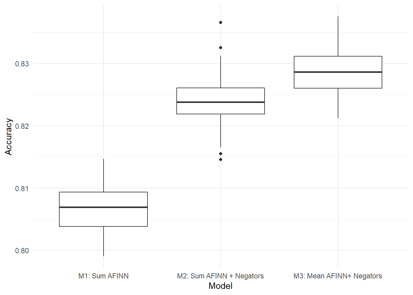

Figure 8.9: Distribution of results for 100 trials of each model. Model 3, Mean AFINN + Negators, outperforms the other models on average.

Figure 8.9 shows the results from 100 trials each of the three models we’ve developed, logistic regressions based on AFINN sum, AFINN sum plus negators, and mean AFINN plus negators. Model 3, mean AFINN plus negators, clearly outperforms the other models on average for this dataset of longer reviews.

We can run the full 5x5 analysis again to get a heat map and box plots and see if it helped.

8.11 Re-Running the Big Analysis

Here we’ll re-run the big analysis using Model 3, mean AFINN plus negators.

First we’ll calculate the mean AFINN score for each review in our full dataset.

afinn_mean <- yelp_data %>%
  select(text) %>%
  rowid_to_column() %>%
  tidytext::unnest_tokens(word, text) %>%
  left_join(afinn) %>%
  group_by(rowid) %>%
  summarise(afinn_mean = mean(value, na.rm = T)) %>%
  mutate(afinn_mean = if_else(is.na(afinn_mean) | is.nan(afinn_mean), 0, afinn_mean))

## Joining, by = "word"

## `summarise()` ungrouping output (override with `.groups` argument)

yelp_data <- yelp_data %>%
  bind_cols(afinn_mean) %>%
  select(-rowid)
  
yelp_data <- yelp_data %>%
  mutate(buts = stringr::str_count(text, "but "),
         nots = stringr::str_count(text, "not "),
         buts_nots = buts + nots) %>%
  mutate(afinn_mean = if_else (is.na(afinn_mean), 0, afinn_mean))

Our results, shown below in Figure 8.10, are promising. Accuracy seems to be higher across the board, and while there are some darker patches in the centre, there doesn’t seem to be a drop-off as word length increases.

results_model3 %>%
  ggplot() +
  geom_tile(aes(x=word_qtile, y=num_qtile, fill=accuracy)) +
  scale_x_continuous(breaks = 1:num_qtiles, 
                     labels = paste0("Q",1:num_qtiles,": ",qtiles, "-",lead(qtiles)) %>% head(-1)) +
  scale_y_continuous(breaks = 1:num_qtiles,
                     labels = (2*round(1:num_qtiles * minn/num_qtiles))) +
  labs(x = "Review Word Length by Quantile",
       y = "Number of Reviews",
       fill = "Accuracy")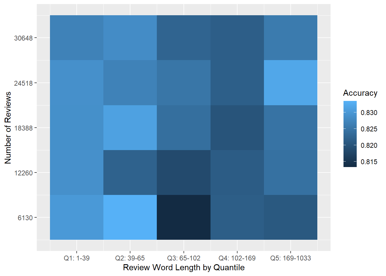

Figure 8.10: Heat map of average accuracy for Model 3. Each cell shows average accuracy for 30 trials on random data subsets.

The results are even more promising when we compare them to those from Model 1. Figure 8.11 shows Model 1 and Model 3’s results side by side, and the difference is dramatic: Model 3 gives better mean predictions across all subsets, and the differences are dramatically positive for longer reviews.

results_comp <- results_oldmodel %>%
  left_join(results_model3 %>% rename(accuracy_m3 = accuracy)) %>%
  mutate(diff = accuracy_m3 - accuracy) %>%
  select(-pct_true_pos)

results_comp %>%
  pivot_longer(cols = c("accuracy", "accuracy_m3"), values_to = "accuracy", names_to = "model") %>%
  ggplot() +
  geom_boxplot(aes(x=as.factor(word_qtile), y = accuracy, fill = model)) +
  theme_minimal() +
  scale_x_discrete(breaks = 1:num_qtiles, 
                     labels = paste0("Q",1:num_qtiles,": ",qtiles, "-",lead(qtiles)) %>% head(-1)) +
  labs(x = "Review Word Length by Quantile",
       y = "Accuracy",
       fill = "Model") +
  scale_fill_discrete(labels = c("M1: Sum AFINN", "M3: Mean AFINN + Negators")) +
  theme(legend.position = "bottom")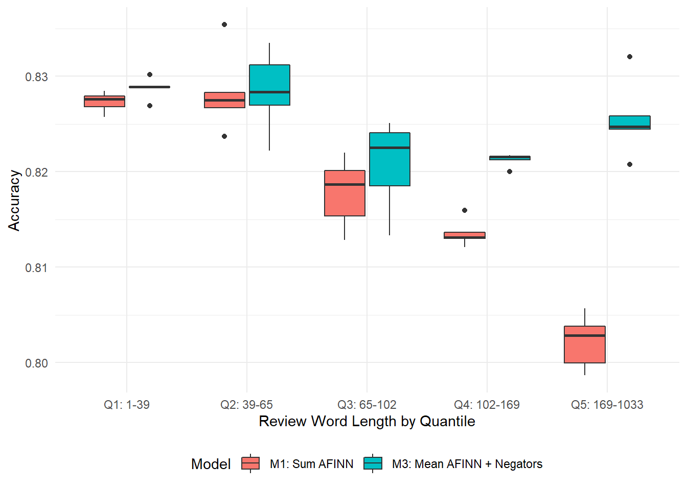

Figure 8.11: Comparing average accuracy rates for Model 1 and Model 3. Model 3 gives better on-average predictions for reviews of all word lengths, and some improvements are dramatic.

Moving Model 3 to use mean AFINN and the number of negators seems to be a Pareto-improvement over Model 1. Model 3 works about as well for all review lengths, and long reviews are about as easy to predict as short ones. As with Model 1, Figure 8.10 shows that Model 3 seems to work about as well for smaller groups as it does for larger groups.

8.12 Conclusion

In this section we looked into last section’s strange finding that longer Yelp reviews led to worse predictions using Model 1, a logistic regression on AFINN sentiment. After a qualitative review of some misclassified long reviews, we looked into two hypotheses for what might be confusing AFINN: that longer reviews might use more negations, and that longer reviews might have lower readability scores. We didn’t find any strong connection with readability scores, but we did find that longer reviews use more negations like “but” and “not.” This led us to suspect that including the number of negations in our regression might improve the model. We also found that longer reviews tend to have slightly higher scores and that score variance seems to increase with length. This suggested that a normalized AFINN score based on a review’s length might be more reliable.

We built and tested two new models. Model 3 performed the best, and improved on Model 1 across all data subsets and did especially well on longer reviews (see Figure 8.11). Model 3used a logistic regression based on a review’s mean AFINN score and its number of “buts” and “nots.” We also improved our model evaluation by using a process similar to cross-fold evaluation, running it 30 times on each data subset using random test/train splits and taking the average accuracy across all trials.

We’ve shown that you can build a model that is roughly 82.5% accurate at predicting Yelp ratings using fast and simple models (AFINN sentiment, logistic regression) with insights from qualitative analysis of the data (counting negators, switching to mean AFINN). The models take only a few lines of code, run in seconds, and are completely supervisable and interpretable.

We’ve also shown two things about using Yelp review text as input data. First, ceterus paribus, review length is not a significant issue when predicting Yelp ratings. Second, our models’ accuracy didn’t change meaningfully based on the number of reviews we used as inputs. Our models were robust across the entire range we considered, from around 6,000 input reviews to around 31,000.

8.13 SessionInfo

sessionInfo()

## R version 4.0.2 (2020-06-22)
## Platform: x86_64-w64-mingw32/x64 (64-bit)
## Running under: Windows 10 x64 (build 18363)
## 
## Matrix products: default
## 
## locale:
## [1] LC_COLLATE=English_Canada.1252  LC_CTYPE=English_Canada.1252   
## [3] LC_MONETARY=English_Canada.1252 LC_NUMERIC=C                   
## [5] LC_TIME=English_Canada.1252    
## 
## attached base packages:
## [1] stats     graphics  grDevices utils     datasets  methods   base     
## 
## other attached packages:
##  [1] beepr_1.3         sylcount_0.2-2    ggridges_0.5.2    vip_0.2.2        
##  [5] glmnet_4.0-2      Matrix_1.2-18     lubridate_1.7.9   tictoc_1.0       
##  [9] discrim_0.1.1     yardstick_0.0.7   workflows_0.2.0   tune_0.1.1       
## [13] rsample_0.0.8     parsnip_0.1.4     modeldata_0.0.2   infer_0.5.3      
## [17] dials_0.0.9       scales_1.1.1      broom_0.7.0       tidymodels_0.1.1 
## [21] textrecipes_0.3.0 recipes_0.1.13    tidytext_0.2.5    forcats_0.5.0    
## [25] stringr_1.4.0     dplyr_1.0.2       purrr_0.3.4       readr_1.3.1      
## [29] tidyr_1.1.1       tibble_3.0.3      ggplot2_3.3.2     tidyverse_1.3.0  
## 
## loaded via a namespace (and not attached):
##  [1] colorspace_1.4-1   ellipsis_0.3.1     class_7.3-17       fs_1.5.0          
##  [5] rstudioapi_0.11    farver_2.0.3       listenv_0.8.0      furrr_0.1.0       
##  [9] audio_0.1-7        SnowballC_0.7.0    prodlim_2019.11.13 fansi_0.4.1       
## [13] xml2_1.3.2         codetools_0.2-16   splines_4.0.2      knitr_1.29        
## [17] jsonlite_1.7.0     pROC_1.16.2        dbplyr_1.4.4       compiler_4.0.2    
## [21] httr_1.4.2         backports_1.1.7    assertthat_0.2.1   cli_2.0.2         
## [25] htmltools_0.5.0    tools_4.0.2        gtable_0.3.0       glue_1.4.1        
## [29] Rcpp_1.0.5         cellranger_1.1.0   DiceDesign_1.8-1   vctrs_0.3.2       
## [33] nlme_3.1-148       iterators_1.0.12   timeDate_3043.102  gower_0.2.2       
## [37] xfun_0.16          globals_0.13.0     rvest_0.3.6        lifecycle_0.2.0   
## [41] future_1.19.1      MASS_7.3-51.6      ipred_0.9-9        hms_0.5.3         
## [45] parallel_4.0.2     yaml_2.2.1         gridExtra_2.3      rpart_4.1-15      
## [49] stringi_1.4.6      highr_0.8          tokenizers_0.2.1   foreach_1.5.0     
## [53] lhs_1.0.2          lava_1.6.8         shape_1.4.5        rlang_0.4.7       
## [57] pkgconfig_2.0.3    evaluate_0.14      lattice_0.20-41    labeling_0.3      
## [61] tidyselect_1.1.0   fabricatr_0.10.0   plyr_1.8.6         magrittr_1.5      
## [65] bookdown_0.20      R6_2.4.1           generics_0.0.2     DBI_1.1.0         
## [69] mgcv_1.8-31        pillar_1.4.6       haven_2.3.1        withr_2.2.0       
## [73] survival_3.1-12    nnet_7.3-14        janeaustenr_0.1.5  modelr_0.1.8      
## [77] crayon_1.3.4       rmarkdown_2.3      grid_4.0.2         readxl_1.3.1      
## [81] blob_1.2.1         reprex_0.3.0       digest_0.6.25      munsell_0.5.0     
## [85] GPfit_1.0-8